Reflections on the scientific path leading to the discovery of a young transiting planet in a debris disk

[ Here is a guest blog cross-post from my friend and colleague Dr. Jonathan Gagné about our recent work on the discovery of AU Mic, written much better than I ever could.  Original post here: https://jgagneastro.com/2020/06/26/au-mic-b-a-new-exoplanet-in-orbit-around-a-remarkable-nearby-star/ ]

AU Mic b: A New Exoplanet in Orbit Around a Remarkable Nearby Star

By Dr Jonathan Gagné

I’m a research advisor at the Planétarium Rio Tinto Alcan of Espace pour la Vie, and I’ll keep you updated with some of our original research here. In this post, I will tell you about the recent discovery of an exoplanet named AU Mic b. This discovery comes from a long collaboration with Dr. Peter Plavchan, associate professor at George Mason University, led since 2010. I joined Plavchan’s team in 2014, and helped them analyze the data that led to the discovery of this new exoplanet.

This blog post is also available in French here.

An illustration of AU Mic b, a new Neptune-sized exoplanet. Credit: NASA’s Goddard Space Flight Center/Chris Smith, USRA

The name of this exoplanet, AU Mic b, is the same as that of its host star AU Mic, except we added a small "b" next to it. This is how we name exoplanets in astrophysics, a convention endorsed by the International Astronomical Union, who are the authority on the naming of astrophysical bodies. This practice stems from binary stars nomenclature; for example, Alpha Centauri is a binary star, and we name its two stellar components Alpha Centauri A and Alpha Centauri B. We use capital letters for stars, and lowercase letters for exoplanets. If we discover a second planet around AU Mic, we'll name it AU Mic c, and so on—we reserve the letter A (capitalized) for the host star, but we usually keep it implicit rather than naming it AU Mic A.

An illustration of the star AU Mic and its debris disk. Credit: NASA’s Goddard Space Flight Center/Chris Smith, USRA

Before we talk more about the exoplanet AU Mic b, I would like to tell you more about its parent star because it is a special one. Its name, AU Microscopii if we write it down in its entirety, comes from the Microscopium constellation where it can be found. We generally name the brightest star of a constellation with the Greek letter alpha (α Mic), the second one with beta (β Mic), and so on. However, the detailed rules are more complicated than this, especially for the fainter stars of a constellation. AU Mic is far from the brightest star in the Microscopium constellation, and that's why its name doesn't begin with a Greek letter. The Microscopium constellation is located in the Southern Hemisphere, but AU Mic can still be seen from Québec with a telescope, in late August and September evenings.

AU Mic is a young star, aged only about 24 million years, compared to our Sun's 4.6 billion years. We know AU Mic's age because it is part of the "β Pictoris moving group" a giant "stream" of stars that move together in space, and were born from the same molecular cloud. I talk more about these stellar groups in my first blog post—I spend a lot of my time studying them!

A visualization of all known stars in the β Pictoris moving group, compared with the position of the Sun, on which the green circles are centered. The green circles have radii between 10 and 100 light years. After approaching the regroupment of stars and moving around it, I stopped the camera and turned on time to view where the stars are moving towards in the upcoming few million years. AU Mic is part of this group of stars, born together but not bound to each other gravitationally. A higher-resolution version of this video is available here.

AU Mic is smaller than the Sun, with about 75% of its size, and half of its mass. We sometimes call such small stars red dwarfs, because they have a cooler temperature, and that gives them a redder color. They are also sometimes called M dwarfs or M stars in technical jargon, and they are popular stars for the search of exoplanets, for a few reasons.

First, they are very common. The physics inherent to the process of stellar formation causes about half of all stars to be born with masses smaller than half that of the Sun (i.e. M dwarfs). The fact that small stars are ubiquitous means that we can hope to find a larger number of exoplanets in total if we consider them in our searches.

Second, the fact that these stars are smaller, less massive, and dimmer makes them great for the detection of exoplanets. The transit method, whereby we wait for a planet to pass in front its star and make it dimmer,  gets us a better sensitivity to small planets when the star is physically smaller. This is true because it is the ratio between the size of the planet and its parent star that dictates how much dimmer the star becomes during a transit event.

This transit method is represented in the video below, where we see the brightness changes caused by planets of different sizes. When we use this method to detect exoplanets, we don't actually see the surface of the star, because it is too far away from us: all that we see is a tiny point of light, which brightness goes down slightly during the transit.

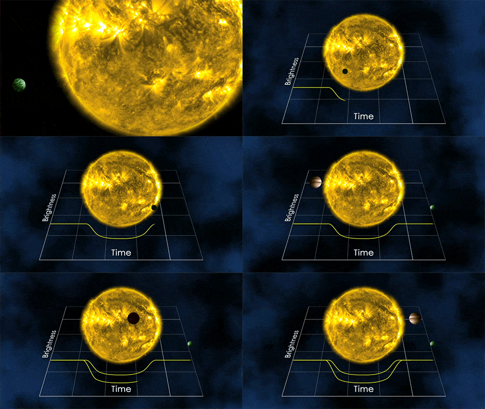
Representation of an exoplanet transit. Larger planets, or smaller stars, will cause a more easily detected change in brightness. Credit: NASA's Goddard Space Flight Center

It is not always possible to detect exoplanets with the transit method, because their orbit needs to be aligned correctly for us to see the planets pass in front of their stars. The transit method also has benefits, however: it allows us to detect exoplanets at very far distances from us. This is why NASA's Kepler mission was so prolific in discovering exoplanets. The Kepler space telescope stared at one patch of the sky for more than 3 years and discovered over 2,300 exoplanets, more than half of all confirmed exoplanets !

A visualization of all exoplanet systems discovered by the Kepler space telescope, over time, and compared with the Solar System planets. Orbital periods and the sizes of exoplanet orbits are to scale, but the sizes of exoplanets are not displayed to scale, otherwise Earth-sized planets would be too small to see them. The exoplanet colors are representative of their expected temperatures, as indicated by the legend. As you can see above, Kepler identified many exoplanets in tight orbit around their star with short orbital periods. This is just because they are easier to find as they transit more often, and it does not mean that all exoplanets have orbits tighter than the Solar system on average. Credit: NASA, Ethan Kruse, music by Kevin MacLeod

Another method often used to detect exoplanets is called the radial velocity method. When an exoplanet orbits around its star, it pulls on the star and causes the star to wobble around a little bit. We can observe that from Earth with our instruments, because the Doppler effect causes the light to become just slightly bluer when the star moves towards us, and slightly redder when it moves away from us. This is analogous to the sound Doppler effect, causing a change of pitch in the sound of a car that moves towards or away from us.

The radial velocity method is what allowed us to discover the first exoplanets around “normal” stars (some exoplanet candidates were found around pulsars a bit before that). Paul Butler, my office neighbor and fellow coffee nerd during my first postdoc at Carnegie Institution for Science in Washington, D.C., is one of the pioneers of the radial velocity method. He likes to recount how his team used a device called an iodine gas cell at the telescope to calibrate their instrument while searching for exoplanets back in the 1990s, and how they were wary that breaking the gas cell would be extremely dangerous.

An illustration of the radial velocity method to detect exoplanets. Credit: NASA, “5 Ways to Find a Planet”

Once again, smaller stars are good for exoplanet detection with the radial velocity method. The intensity of the star's wobble, and therefore the color shift of its light, depends on the ratio between the mass of the planet and that of its star. Therefore, using the same instruments and telescope, we will be able to detect planets of a smaller mass around stars of a smaller mass.

There is, however, one problem that muddies the benefits of exoplanet detection around small stars: small stars are often "hyperactive", which means that they often flare, have lots of stellar spots, and magnetic storms that cause large and random flashes of visible light, UV and X-ray at their surface. This really complicates the detection of exoplanets, because these random events "pollute" the signal of potential exoplanets, and make our data a lot noisier.

The younger stars are even worse in this regard: for reasons we will not get into this time, young stars tend to rotate faster, and that causes them to have stronger magnetic fields. Magnetic fields are what drive stellar spots, mass ejections and violent storms at their surface, so younger stars with stronger magnetic fields will be even more active. AU Mic is one of the worst possible case scenarios in this regard: it is both small and young. Peter Plavchan likes to call it "Speedy Mic" for this reason, because it is a particularly unstable star that likes to flare a lot.

A visualization of what the star AU Mic A might look like with its large clusters of stellar spots and magnetic storms causing bright flashes in visible light, as well as UV and X-ray. Credit: NASA’s Goddard Space Flight Center/Chris Smith, USRA

AU Mic is also really cool (and problematic) for yet another reason: it has a massive disk of debris around it. These debris are the result of planetary embryos, also called protoplanets, smashing into each other and getting blown to smithereens. This disk was discovered in 2005, and has been studied extensively since then. Researchers even found that clumps are moving away from the AU Mic at about 40,000 kilometers per hour in its debris disk! It is still unclear to this day what causes this.

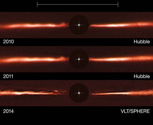
Hubble and VLT images of the AU Mic disk. These images show the debris disk at distances up to about 60 astronomical units from the star (one astronomical unit is the Sun-Earth distance), and how its structure changes over time. Credits: NASA, ESA, ESO, and A. Boccaletti (Paris Observatory)

A study led by Cail Dailey using the Atacama Large Millimeter Array Observatory (ALMA) also looked at AU Mic's debris disk much closer in, and saw that some debris are being stirred, causing the disk to be thicker at separations from the star between 20 and 40 astronomical units. They think this is caused by either large planetary embryos, or a hidden exoplanet with less than about twice the mass of the Earth.

An image of the inner debris disk of AU Mic taken by ALMA. This image is zoomed in a lot more compared to the previous ones obtained with Hubble and VLT/SPHERE. Credit: Joint ALMA Observatory, ESO, AUI/NRAO, NAOJ, and Cail Daley (Van Vleck Observatory)

Now, this is a really cool star (in all senses of the word), but it is very hard to search for exoplanets around it because it is super active. We needed something to get past these problems of stellar activity if we hoped to open up the study of exoplanets around small stars in general with the radial velocity and transit methods. One strategy to do this is to stick with the radial velocity method, but look at the star's infrared light rather than its visible light. The signature of stellar activity does not impact infrared light as much as visible light, and the signature of an exoplanet is still apparent in the infrared. However, infrared detectors are a younger technology, making them a lot more expensive and less precise. It is also a lot harder to get a good calibration for these instruments, and this is required to precisely measure a star's color shift as it wobbles around.

This is where Peter Plavchan and his team come in: since about 2010, Peter started collaborating with NASA's Jet Propulsion Laboratory to develop such calibration devices. They built a device called a methane isotopologue gas cell, analogous to the iodine gas cell Paul Butler used, except that it is designed for infrared light (and it is also way less dangerous, thankfully). Peter's team also worked on developing a device even more precise, but way more expensive, called a near-infrared laser comb.

The methane gas cell we used at the Infrared Telescope Facility to calibrate our measurements. The gas cell itself is the transparent cylinder at the center of the photo; it is attached in front of our camera, and will therefore sit between the telescope and the camera. The light we receive from a star will pass through this transparent device, and get imprinted with the unique signature of the methane molecules contained in the gas cell, before making its way to the camera. These molecular fingerprints will serve as a calibration for our scientific measurements.

As soon as Peter got his hands on his methane isotopologue gas cell, he placed it on an instrument called CSHELL at the Infrared Telescope Facility (IRTF) in Hawaii. He began observing some stars near the Earth with his team, focusing on those which exoplanets were inaccessible to visible-light instruments: small stars, and in particular young ones. As you can imagine, AU Mic was one of the first stars they pointed the telescope at, back in 2010.

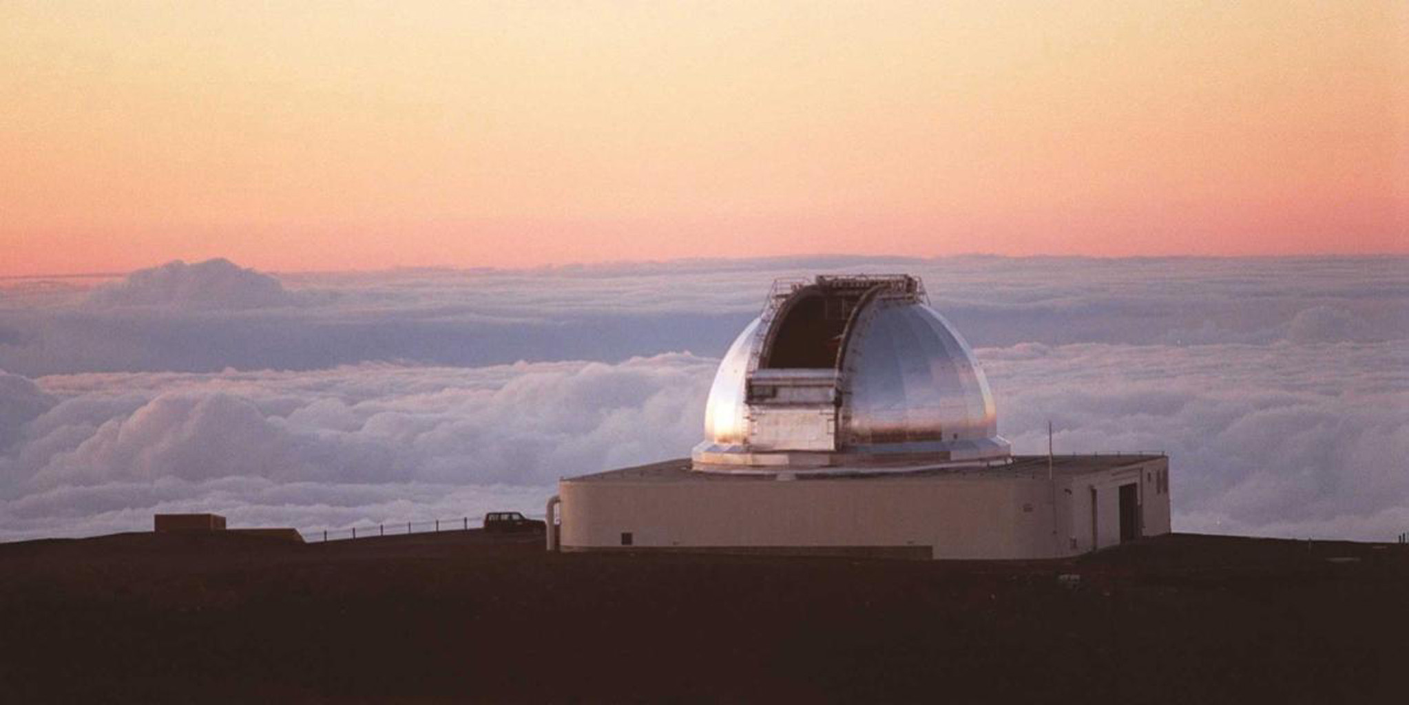
The IRTF telescope, on the Mauna Kea volcano in Hawaii. The observatory literally sits above the clouds. Credit: NASA, JPL

It's only in 2014 that I joined Peter Plavchan's efforts in this project. I was 4 years into my Ph.D., working on the detection of brown dwarfs in young groups of stars, like the β Pictoris moving group with René Doyon and David Lafrenière at Université de Montréal. I applied to an online contest for a 6-months scientific exchange with researchers at the Infrared Processing and Analysis Center (IPAC) at Caltech, and to my delight, I obtained an assignment with Peter Plavchan to work on the detection of exoplanets. So I moved to Pasadena, and excitingly started working with Peter and his team during that next summer. As part of this project, I went to IRTF a few times and observed many stars, AU Mic part of those, with CSHELL and Peter's methane isotopologue gas cell.

Apart from helping with the telescope observing, I spent much of my time in Pasadena writing computer codes to transform the raw data the CSHELL camera gave us into measurements we can use and interpret. This may sound surprising when you are used to taking pictures with a commercial camera, but images that come out from scientific cameras require a lot of work before we can hope to obtain a final product. In this particular case, the final product we obtain for every star, and every night spent at the telescope, is a single measurement of how fast the star is moving towards us, or away from us (this is what a radial velocity measurement is). Pasadena is also where I discovered Copa Vida's single-origin espresso shots, which began a whole other journey for me!

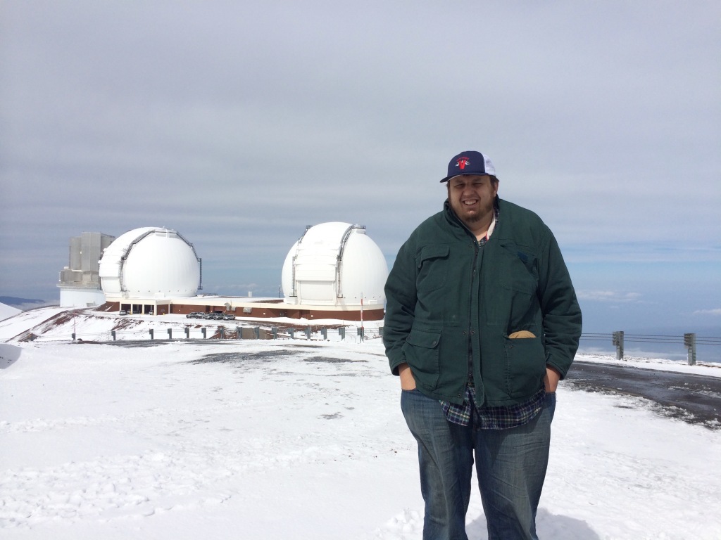
Peter Plavchan and I, staring at the Sun with the Keck telescopes in the background. This is the view we had when arriving at the IRTF telescope, located behind the camera. Photos by myself and Peter Plavchan

When I came back to Montreal after this delightful experience in Pasadena, the work was far from being done—research projects like this one routinely require decades of work, especially when new instrument technologies are involved. I kept my collaboration going with Peter Plavchan, and continued analyzing CSHELL data, and observing remotely with CSHELL, as one of my several ongoing projects. In 2016, I led the writing of a scientific paper that described our first results with this project. Our instruments were not yet precise enough to detect AU Mic b, but we ruled out the presence of a planet more massive than Jupiter in tight orbit around AU Mic. Peter Gao, also part of Peter Plavchan's team during my stay in Pasadena and now a close friend, led another scientific paper in 2016 where he described the algorithm he built to take in my calibrated CSHELL data, and transform it into a radial velocity measurement (yes, this science is so complicated that it required two computer codes, mine and Peter Gao's).

Shoveling snow was part of the job as we got caught in a snowstorm during one of our 2017 observing runs at the IRTF telescope (seen here in the photo). Photo by Peter Plavchan

By the time we published both our 2016 papers, a new and improved infrared camera came up at IRTF. This one, called iSHELL, is similar to CSHELL in what it does, except it is so much better, and in particular more precise. We immediately started using it, and soon after the team started gathering enough data, I flew to Missouri state where Peter Plavchan was now a faculty member at Missouri State University. We sat down with his new student Bryson Cale, and spent the week developing new computer codes for the iSHELL camera in a hack-a-thon style week. They both later came back to visit me in Washington, D.C. during my first postdoc, where we worked more on the computer codes.

Once we started gathering iSHELL data, it did not take long before Peter Plavchan noticed something weird about AU Mic. He emailed us in fall 2016 to tell us that he thought there might well be first signs of an exoplanet hiding in our data. However, this would have been a dangerous claim to make publicly, especially given that we were venturing in an unexplored territory with applying the infrared radial velocity method to an exceptionally active star. We needed to be absolutely certain that what we were seeing was an exoplanet, so we needed to keep observing it as often as possible.

A view of the IRTF telescope's primary mirror from inside the dome. Photo by Peter Plavchan

As we gathered more data, the signal became gradually clearer that there was an exoplanet similar to Neptune around AU Mic. But then, NASA launched the TESS space telescope, and it too observed AU Mic! The TESS mission stared at many stars close to the Sun, hoping to detect exoplanet transit events, like those that we described earlier. As is often the case with NASA missions, TESS data is available to everyone soon after it is observed, and it becomes a gold mine for any researcher to dig in. Obviously, Peter started looking for our new candidate exoplanet AU Mic b in the data that TESS gathered for the star AU Mic, and he found exactly what he was looking for: two transit events seemingly caused by a Neptune-sized exoplanet!

The transit signal also indicated that AU Mic b orbits its star every 8.5 days. This is an extremely short orbital period! Imagine if the Earth orbited around the Sun that fast: our year would only last 8.5 days. AU Mic b orbits so fast because it is very close to its star, at 0.07 astronomical units, only 7% of the distance between the Earth and the Sun. The radial velocity data we have in hand also indicates that the mass of AU Mic b is smaller than 3.4 times that of Neptune, and TESS data indicates that its size is almost exactly the same as Neptune. Interestingly, TESS data also shows hints of a possible second planet, at 0.13 astronomical units from the star (almost twice as far from its star as AU Mic b), and twice the size of the Earth. However, we will need more data to be sure, especially when working with a star as noisy and unstable as AU Mic.

This is a really cool discovery, not only because it opens the door to more research for exoplanets around young and small stars. The fact that AU Mic is so young means that we are catching the exoplanet AU Mic b in the first moments after it formed. Some researchers think it may have formed a bit further from its star, at about 10 astronomical units, and then migrated inwards. If that is true, it means that it must have migrated fast, because it already landed as its current location when the star is still only about 24 million years old.

A video based on a computer simulation, showing how a planet may form inside the disk of a star, causing spiral waves in the disk, and later migrate inwards closer to the star. Credit: Ximena S. Ramos and Pablo Benítez-Llambay

This discovery also gives us a complete picture of what a debris disk looks like in a system that just completed forming an exoplanet like AU Mic b. We know that exoplanets form inside disks around young stars, so we can now look at AU Mic's disk and wonder what imprints AU Mic b might have left on the disk. We can also hope to observe soon exactly how the intense UV and X-ray radiation of AU Mic, as well as its stellar wind, are affecting the atmosphere of AU Mic b. We think that these phenomena could cause the atmosphere to be eroded away. This is an important question because it will determine how hostile to life stellar activity may be for rocky exoplanets around small stars (we think AU Mic b is made of gas, like Neptune).

Another reason why this discovery is so cool is that AU Mic is really not that far from us: it is only 32 light years away, what we can safely call our galactic backyard. It is indeed one of the closest stars to us in the whole β Pictoris moving group, as can be seen below:

A visualization of all known stars in the β Pictoris moving group, compared with the position of the Sun, on which the green circles are centered. The green circles have radii between 10 and 100 light years. The camera moves around the β Pictoris moving group, and then I gradually increase the brightness of AU Mic to show where it is located: it is one of the β Pictoris moving group stars nearest to us. A higher-resolution version of this video is available here.

This system is so close to us that AU Mic b is one of the closest exoplanets we currently know! In fact, only 37 of the currently confirmed 4,171 planetary systems compiled on the NASA exoplanet archive are closer to us than AU Mic. But yet again, an image is worth a thousand words, and a video is worth a thousand images:

A visualization of the AU Mic system location compared with the position of the Sun, on which the green circles are centered. The green circles have radii between 10 and 100 light years. After a few seconds I turn on the locations of all 2,979 currently known and confirmed exoplanet systems for which we know the precise distance from the Sun (required to determine their 3D position). Notice how some of the exoplanet systems form square patterns in the sky when the camera is close to the Sun, at the seventh second of the video near the center of the frame: those are the shapes of the Kepler detectors, back when it always stared in the same direction during its main mission. When we move away from the Sun, we can better see how known exoplanets are located either relatively close to the Sun, or in the direction where Kepler stared. A higher-resolution version of this video is available here.

Peter started the long process of writing up and submitting a scientific paper to the journal Nature, which was finally published this June 24th. This discovery caused quite the media sensation, and even trended on CNN!

Now the science does not end here: Peter got busy teaming up with scientists around the world before publishing his Nature paper, to begin further investigations of this new planetary system. This led to five(!) additional scientific papers, all timed to also become public on June 24th. Four of these teams measured the obliquity of AU Mic b—the tilt between its rotation axis and the axis of its orbital motion, see this video for more explanations—and they all found that the planet's spin axis is aligned with its orbital axis. This is evidence that it indeed formed from AU Mic's protoplanetary disk, and likely did not suffer a cataclysmic collision with other planetary embryos.

There are still many unknowns about how planets form, so discovering young systems like AU Mic b is important to challenge our expectations and refine our understanding of this process. Each one of these discoveries provides us with a "photography" of what a given system may look like at a given age. Remember that one million years is very short at the astrophysical scale, so we cannot wait to see how AU Mic b will evolve, and we need to instead find another similar but slightly older system if we hope to constrain exactly what will happen next in the life of AU Mic b.

One of the five teams mentioned above, featuring other members of the Institute for Research on Exoplanets at Université de Montréal here in Québec, also measured the strength of the magnetic field of the star AU Mic, and how it varies with time. They used this to better understand how the star's activity affected the radial velocity measurements.

Another scientific team tried to measure the atmospheric composition of AU Mic b with a method called transit spectroscopy, but the star was so active that it prevented them from being able to measure a useful signal. NASA's upcoming James Webb Space Telescope (JWST) will probably be able to do this successfully.

Finally, another one of the scientific teams built computer simulations to better understand how AU Mic's stellar wind may affect the atmosphere of its exoplanet. They found that stronger winds will tend to compress the planet's atmosphere, and make it harder to measure its composition with our instruments. They also made predictions about what the transit would look like at a specific wavelength of light (i.e. a color of light). Measuring AU Mic b's planetary transit with an instrument designed to see this specific color only will shed more light on how strong the stellar winds of AU Mic are, and whether AU Mic b's atmosphere is getting eroded or not by the star's violent UV and X-ray emissions.

NASA got so excited about this discovery that, on top of all the nice visualizations they made for AU Mic and its planet, they also created this awesome poster:

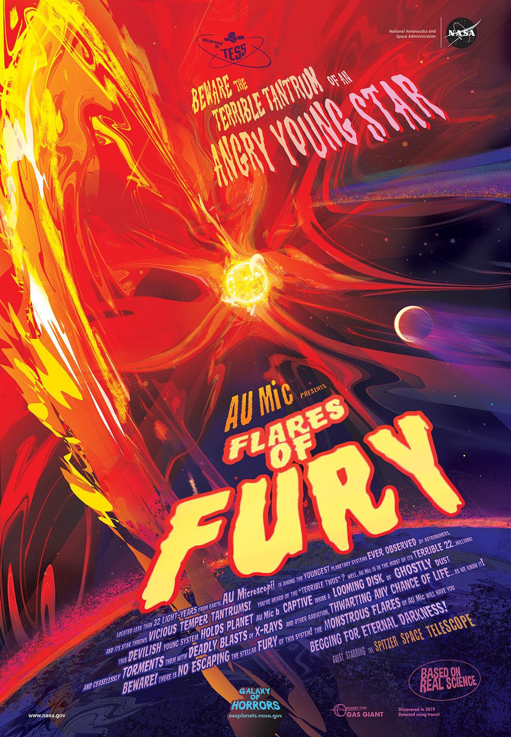
A promotional poster of the exoplanet AU Mic b. Credit: NASA-JPL/Caltech

I'm super proud to have helped Peter and his team with this discovery, but I also want to emphasize how this is the result of such a long haul, sustained commitment on his part. Peter not only put together the technology to do this and taught several students how to use it along the way (including myself back in 2014), he also led the decades-long observations of AU Mic, and jumped through many hoops to publish this discovery, across many moves, position changes, and obviously, a world pandemic. I sure hope he will line his walls with that poster!

I would like to thank Peter Plavchan, Marc Jobin, André Grandchamps and Marie-Eve Naud for their comments.

 

 

A proposed COVID Cohort model for re-opening college campuses when they reopen

Disclaimer: I am not an infectious diseases expert.  This proposal is not to be construed as an official recommended course of action. This proposal has not been reviewed by infectious disease experts, and this article is a means of seeking feedback from experts and non-experts alike on the viability and likelihood of success of this proposal.

Faculty at George Mason were asked for any input on the re-opening models being trade-studied for fall 2019.  This is my edited response:

A Proposed "COVID Cohort" Model for Re-opening College Campuses in Fall 2020

This proposed cohort model does not eliminate the need for facemasks, cleaning and santitation, and other social distancing measures in common areas as recommended by draft CDC guidelines.  This model supplements those approaches.  This model is under the assumption that we re-open campus to a significant fraction of students and staff; whether or not we re-open campus and under what criteria is beyond the scope of what is discussed here.

The goal of social distancing is to minimize the number of close social interactions we have to reduce the rate of community spread of COVID-19.

A plan to re-open a college campus should maintain similar goals.

Under a normal academic schedule at a typical US college, a college student, let's call her Alice, may take 5 classes of an average of approximately 30 students each.  Overlap of students enrolled between classes, particularly for freshman taking general education courses, can be a small number or zero.  In other words, if Alice and Bob both take ENG 101 together, the odds of them taking a second class together is low. Thus on a weekly basis, a single student like Alice can come into close social contact in their courses with approximately 150 peer students on average (and likely more given large lectures). In the presence of viral community spread, if Alice contracts COVID-19, Alice can potentially spread coronavirus in normal (pre-COVID-19) classrooms to approximately 150 (or more) other students.

[Edit: A recent network study by Cornell highlights that a single student can via three student interactions come into indirect contact 98% of a college student population under the pre-coronavirus status qup: https://www.insidehighered.com/news/2020/04/14/sociologists-say-their-findings-student-interconnectedness-suggest-caution-needed ]

If, however, a University implements a "cohort" model - a group of students that take classes together - we can reduce the rates of coronavirus spread by factors of approximately up to five in this toy model.  If instead Alice takes the same 5 classes with the same 30 students, and if Alice contracts coronavirus, Alice can now only spread coronavirus to 30 students instead of 150 within the classroom setting.

Thus, I recommend college campuses consider a COVID cohort option for re-opening in the fall.  We want to maximize the number of classes students take together in person in common to minimize the number of distinct physical social interactions a student has. This is entirely aligned with the draft CDC guidelines for childcares and schools re-opening:

"Ensure that student and staff groupings are as static as possible by having the same group of children stay with the same staff(all day for young children, and as much as possible for older children).  

Restrict mixing between groups."

This will be a challenge to implement - students are currently given the freedom to choose classes independently to suit their schedules, and in fact registration has already begun at many campuses for the fall semester.  However, we know when freshman take general education courses, many have similar courses in common albeit in different sections or large lectures.  Additionally, for upper-class students with declared majors, many take classes inside their major together.  Unfortunately, we have already passed the time when students have started registering for classes, and so we may limited to identifying cohorts from students already enrolled in courses together.

I would like to propose that upper-class students based upon their declared majors and year be placed into cohorts by academic advisors familiar with students academic progress to  take the same courses together for the fall 2019 semester, and to request students minimize or take online only classes for the classes that they can not take with their cohort.  For example, junior physics majors could be a "cohort", and if they take any classes outside of their major-year cohort, they must take them virtually online.  In addition, to all extents practical, cohorts should take all of their classes in the same physical classroom, since the virus can also spread via surfaces.

Similarly, for freshman that have many classes in common, may I propose that their schedules be divided into cohorts based upon general education course sections of ~30 people and their expressed majors or undeclared interests.  Again, if freshman students take non gen-ed classes outside their cohort or declared major, they be required to take those classes virtually or online.  Another cohort could be honors college students, for example, again organized by class year, and college or major for declared students.  Students that live off campus could potentially be given a separate cohort designation from those that live on campus, especially given that students that live off campus are more likely to have additional social/work interactions off campus and outside the campus community. Students can also be given the option of choosing cohorts that are entirely online, particularly students that have underlying conditions or concern of contracting the virus.

To promote the adoption of these student cohorts of ~30 people in size, may I suggest that the face masks a University will hopefully be providing to students be given colors or University symbols of pride or chosen major symbols that let students easily identify when they are among students from their cohort or not.

For freshmen and students living on campus, they could be physically located in dorms aligned by cohort, so that the social interactions of students outside of class will be similar to the students they have in their classes.

The cohort model has been shown to promote retention of students (like in live-and-learn communities), and having students take the same classes together and live together could lead to overall better academic outcomes during these times of a pandemic crisis. Some programs already on campus have identified cohorts (like the honors college).   The cohort model for education for retention and identity building has a strong and positive academic heritage.  Organizing classes / dorms around a cohort model to the practical extent possible could both be touted as a positive education approach in higher ed and have real benefits in limiting virus communal spread.

Additionally, cohort model will help with contact tracing and mitigation for cases that do appear on campus.  Freshman moving onto campus should be encouraged to come to campus two weeks before the start of the semester, and then isolate together in their new cohort.  At the end of the two weeks, they can be tested and begin instruction.

In the era of limited testing capabilities, if a member of a cohort during the semester comes down with coronavirus symptoms or tests positive for coronavirus, the entire cohort can self-quarantine, and be put on required virtual instruction while the rest of campus can continue uninterrupted.  Members of cohorts can be periodically tested for coronavirus as representative samples.

This type of approach would be easier to implement if all professors teaching in person classes also recorded their classes for posting online and for remote participation.  The faculty, which will teach 2-4 classes, can still get infected as well, and spread the virus to all of their students.  So faculty and staff will have to take extra social distancing measures - not handing out printed materials but using digital materials and exams only, for example - to avoid spreading the virus from classroom to classroom.

Finally, elementary schools naturally arrived at the cohort model for organizing student education, by having the same students take the same set of classes, sometimes in the same room with teachers rotating through classrooms.  There is precedent for a cohort model in education in general and higher education specifically.

Understanding Written Science

Forbes and Nature recently published these two articles on the complexity of science writing:

https://www.forbes.com/sites/brucelee/2017/03/26/study-re-emphasizes-if-you-want-to-advance-science-try-explaining-it-more-simply/#61cc0de013ae

http://www.nature.com/news/it-s-not-just-you-science-papers-are-getting-harder-to-read-1.21751

These articles is related to one of my "deep thoughts" about science. Scientists have a need for precise communication to other scientists in order to accurately convey the details of our analysis. As a result, we have developed what are effectively entirely new languages full of technical jargon. Reading a biology paper is completely foreign to me. Even sub-fields within astronomy can read like different "dialects." For example, we can use different words between fields for the same mathematical analysis technique. This article is more about the quality of writing (sentence and word complexity), but the point is related. I'm glad to see that at least some people are attempting to understand this phenomenon and its implications. The need for science communicators (aka "translators") for the general public speaks to my fear of the (growing?) disconnect between scientific progress and the public perception of science. I fear that many of our failures - e.g. global warming, evolution - stem from a failure, or at least an underfunded effort, to communicate (translate) effectively. I'd even go so far as to change the typical formatting of a scientific papers in journals to require as a new standard the inclusion of the equivalent of an "executive summary" for the public - not just an abstract, but something free of jargon and comprehensible to a high school graduate. 

To summarize: The output of science shouldn't be accessible to only a select few who speak a specific "language" that requires years of specialized training to understand. Years of specialized training to undertake said research, sure. But not to understand the gist.

The Superbowl of Astronomy

Over 2400 students, professors, scientists and journalists will gather at the Gaylord Convention center in Grapevine, Texas this week to listen to over 1600 talks, explore exhibit booths, catch up with colleagues, and network.  We're here for the 229th meeting of the American Astronomical Society, referred by space.com as the Superbowl of Astronomy.

I'm bringing four of my students to the conference, and my department colleague, Dr. Mike Reed, is also bringing three of his students.  Springfield, MO is close to the center of the country, so we decided to make the trip to Texas by car - a 7 hour road trip! (for reference, the east coast is a ~16 hr drive; west coast ~24 hr drive, and Chicago ~8 hrs).

 

I'm reminded of this scene from the PhD movie sequel:

 I've apparently reached the PI career stage

To entice you to attend our posters and talks, below is a list of what Dr. Reed, myself, and our research students will be presenting.  Four students (marked below with an *) are applying to PhD programs, so if you are on a grad school admissions committee be sure to talk to them!   Many more of my former students are also going to the AAS meeting, and I look forward to catching up with them, listening to their talks and seeing their posters.

First year masters student, Bryson Cale*, will be giving a talk on Saturday morning (11:10-11:20am, Texas D, Session 403. Extrasolar Planets Detection: Radial Velocity II).  Bryson will present the motivation and first light observations with an isotopic methane gas cell on the iSHELL spectrometer at the NASA Infrared Telescope facility.  Our goal is to measure relative radial velocities of stars to better than 3 m/s precision to search for habitable zone exoplanets around M dwarfs, and to confirm planets discovered by the TESS mission.

Bryson Cale

First year masters student Patrick Newman*, will be presenting a poster on Wednesday (146.10 Extrasolar Planets: Detection Poster Session).  Patrick is working on radial velocity survey yield simulations for input into a future flagship direct imaging mission like WFIRST, HabEx, and LUVOIR. WFIRST will be launching in the 2020s, and HabEx and LUVOIR are under study right now for the 2020 Astrophysics Decadal survey for launch possibly in the 2030s.

Patrick Newman

Senior undergraduate Ryan Hall* will be presenting a poster on Wednesday (146.14 Extrasolar Planets: Detection Poster Session).   Ryan is the current lead of MICRONERVA, an array of small eight-inch telescopes to work robotically and autonomously together to synthesize the light gathering power of a larger telescope.  Ryan will present on the current capabilities and development of the prototype array of four telescopes.  Ryan and I will also be presenting at a splinter meeting for the MINERVA team on Thursday.

Ryan Hall

Senior undergraduate Shannon Dulz* will be presenting a poster on Thursday (245.13 Extrasolar Planets: Characterization & Theory Poster Session) on measuring Transit Timing Variations of two Kepler planetary systems. Shannon developed her own custom code, using a custom transit shape model to speed up the transit fitting process in determining the time of transit midpoint.

Shannon Dulz presenting at a conference in April 2016

Junior undergraduate and computer science major Frank Giddens will be demoing (at Ryan Halls poster) his node.js web server interface to MICRONERVA, complete with Python bridges to the hardware. Watch with us on a webcam as we remotely control the telescope and accessories back in our lab 400 miles away, as long as we don't have any live-demo technical difficulties!

Frank Giddens

Undergraduates John Crooke and Ryan Roessler will be presenting a poster (433.17 Stars of Many Stripes Late Poster Session) on their work with Dr. Reed on the asteroseismology of the subdwarf B star PG 1219+534.

I (Dr. Peter Plavchan, Assistant Professor, Missouri State University) will be presenting a talk on Friday (2:40-2:50pm Texas D Session 320. Extrasolar Planets Detection: Radial Velocity I).  I will be presenting the discovery of a candidate Jovian exoplanet around AU Mic!  The paper is drafted and circulated to co-authors, and will be submitted soon!

My colleague Dr. Reed will be presenting a talk on Wednesday (3-3:10pm Texas 4 Session 130. Variable Stars, Asteroseismology) on his latest research on the asteroseismology of subdwarf B stars.

I'm ready for the kickoff for the astronomy Superbowl!

MICRONERVA - my "moon shot"

I finally updated my research group web page, admittedly more than halfway though a busy semester!   On my web page you can meet the new students in my research group, along with new articles and podcast appearances, and a description of our new masters degree emphasis in astronomy.  Now it is time for a new blog post too!

This past summer MICRONERVA started to take up residence at Baker Observatory.  In this post I will highlight the work of Central Methodist University senior physics major Denise Weigand, and how we went from a drawing on a Powerpoint slide to the built frame for the MICRONERVA prototype enclosure.

Denise was funded as a Missouri SpaceGrant Consortium intern to come work with me at Missouri State University.  I spent most of my summer traveling on the east coast (two immediate family weddings, a couple conferences, etc.), so we had to work remotely.  For that, we used Google+ Hangouts to share screens, audio and video to communicate effectively from a distance.

First, a bit about MINERVA, the "parent" observatory concept behind MICRONERVA.  For a number of years I've been helping with the more complex, larger version called MINERVA.  It's designed to be completely robotic and autonomous after initial setup and regular maintenance:

The basic principle behind MINERVA is to synthesize a larger telescope aperture by combining the light from multiple, smaller telescopes at a lower cost.  The cost of a telescope has a steeper than linear dependence on the telescope primary mirror area:

The cost of single aperture telescopes (red and blue data points) compared to multiple aperture telescopes (green data points).  The solid lines in red and blue indicate approximate power law relationships.  The jump at a diameter of ~1.2 meters marks the transition from the amateur market to the lower demand market that is partially dictated by military expenditures.  From Figure 1 of Swift et al. 2015.

For seeing-limited telescopes there is no loss in angular resolution, which is true at visible wavelengths for any primary mirror larger than ~8-inches in diameter without adaptive optics.  Additionally, the spectrograph shrinks in volume as N^3/2, where N is the number of telescopes, making it a lot cheaper and more stable too. In the case of MINERVA, four 0.7 m telescopes need a spectrograph 1/8^th the volume of a spectrograph for a single 1.4 m telescope.  Thus, one saves costs on both the telescopes and the spectrograph.  And because the spectrograph is smaller, it makes it easier to measure precise radial velocities to hunt for exoplanets.  It's a win-win situation all around.  As far as I know, MINERVA is the first successful on-sky demonstration of this multi-telescope approach for precise spectroscopy.  One of the enabling technologies are fiber optics, which allow us to bring together the light from several telescopes to a single spectrograph entrance slit.

Anyway, back to MICRONERVA.

Upon my arrival at Missouri State University in the fall of 2014, I saw that we had a number of computer controlled CPC800 Celestron Telescopes lying around for educational use.  I also noted that with a simple tip-tilt adaptive optics, light could be effectively coupled from these eight-inch telescopes into special optical fibers called single mode fibers.  In other words, we could build a mini-version of MINERVA - aka MICRONERVA - if we could effectively turn these telescopes into computer controlled autonomous robots.  Additionally single mode fibers provide the ultimate limit in the stable illumination of spectrographs, critical for measuring precise radial velocities.

We decided to start with a prototype of array of four telescopes, but this concept is extremely scalable and even cheaper than MINERVA.  I envision a future array of many hundreds of these telescopes, similar to the HATPI concept by Gaspar Bakos for exoplanet transit searches, but this time for spectroscopy.  I find this is a potentially more cost effective approach for large aperture spectroscopy compared to other concepts such as the Mauna Kea Spectroscopic Explorer:

HATPI concept design

Fast forward to the spring of 2016.  My former student Claire Geneser, now a graduate student at Mississippi State University, managed to get the telescopes to point to a series of targets entirely under the control of a laptop computer:

We still had a number of issues to solve - could we guide at <1 arc-second precision?  Could we control all of these telescope autonomously from a web page?  I'll post about our progress on these challenges at a later date.  We also needed an enclosure to hold the telescopes, something that could open and close on its own.  That is the problem Denise chose to solve.

Denise joined my research group in mid-June of 2016. We had looked into buying a pre-built "dome" like the excellent domes from Astrohaven.  However, at costs of >$25,000, these were beyond the limits of our modest budget.  We were going to have to build one ourselves. Our prototype telescope array will be located at Baker Observatory, shown below:

Baker Observatory, north of Marshfield, MO, the birthplace of Edwin Hubble

In the photo above you can see two traditional telescope domes that are the usual landmark for an observatory.  However, these domes are far more complex than necessary to build an autonomous robotic facility.  Between the lower shutter, dome slit, and dome rotation, three separate motors are needed to open, close and point the dome.  A far simpler approach for autonomy is to design an enclosure that needs only one motor to open and close.  One motor is much easier to program and control than three, even if the end result isn't as exciting as looking at the domes above.

Below is the first sketch Denise and I made of what would eventually be our prototype enclosure in mid-June. This drawing was made with Powerpoint while we talked on Google+ hangouts more than 1000 miles apart:

The first MICRONERVA enclosure sketch.

The design involved the smallest number of exterior surfaces - five - and a single motor to make the design as simple as possible (one of the guiding principles in our design process).  It wasn't our first design, but it was the first design to make sense.  The four shapes inside the triangular room represent the envelops of the four telescopes - e.g., the space they will fill after going through all possible directions they point.  The red surfaces for the roof, the triangles the side walls, and the rectangles some legs to hold the structure off the ground, to prevent moisture wicking and contact with snow in the winter.   The whole thing would be oriented east-west, to enable the largest declination range viewable, at the expense of some east-west horizon obscuration by the triangular walls.

Denise set about her summer turning this sketch into reality.  First up was getting the dimensions right, and here were some sketches that passed back and forth between us.  We started with Powerpoint because it had an easier learning curve than AutoCAD, and let us quickly iterate on ideas.

 

At the end of June, it was time to graduate to three dimensions, which we used Google Sketchup to get started:

We also started thinking about how the roof would roll of and on.  We had already settled on this excellent motor drive from MVO Controls:

Denise made a parts list, and readied to go to Lowe's and Home depot to acquire the wood we needed.  We decided to start with wood rather than aluminum or metal, since it was more forgiving of us to make mistakes, and it was cheaper too.  We'd learn our mistakes on this prototype, which would make things easier the second time around if we went for more permanent and expensive materials.

We next enlisted the help of our campus mechanical engineer, Brian Grindstaff, to help with some of the engineering logistics - e.g. building the floor like a deck with joists and slatted cross-beams and such.  For the first three weeks in the July heat, Denise and Brian build the decking floor and roof frame in the loading dock outside our departments building.  Having it on campus made it easier to work on every day, but then we'd have to transport it out to Baker Observatory, a 40 minute drive!

Brian helped Denise put her design into AutoCAD, and pick the roofing material, wheels, wheel channel. and many other practical aspects of our design under Denise's guidance.

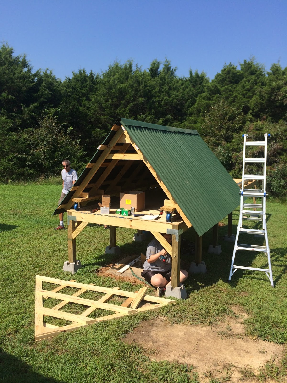
By August 8th, Denise and I used Google maps to plot a final location for the enclosure at Baker Observatory, next to my colleague Dr Mike Reed's robotic 16-inch telescopes, BORAT.  It was ready to ship! The night prior Denise and I went to Baker Observatory with wooden stakes, string and a level, and staked out the position of the enclosure and made sure it'd be on ground that was level enough to be fixed with a shovel and some sweat.

To get the enclosure to Baker Observatory, we made the enclosure relatively easy to disassemble into three pieces - the roof, the deck floor, and the extension for the rails when the roof is "open".  We transported it on one of my students 16'x8' trailers.

The morning of August 9th, we loaded the enclosure onto the trailer.  We left as early as possible to beat the Southwest Missouri summer heat and humidity.  I also recruited my entire research team to help with the lifting and moving.  We had gotten good at this teamwork, because back in June we built a fence at the observatory.  We used reclaimed wood from a long fence in my subdivision that had been torn down and replaced after a pickup truck crashed through it:

Missouri State physics majors Joe Huber and Ryan Hall

Fence building at Baker Observatory in June of 2016 to help with car headlights during our public viewing nights.  Featuring Missouri State CS majors Frank Giddens and America Nishimoto, physics major Laura Ketzer, and Dr. Mike Reed.

Unloading the enclosure pieces on August 9th took a lot of work, and we were all very dehydrated by midday:

Lifting the roof onto the platform was the hardest part.

Denise Weigand next to her roll-off roof enclosure design built and installed!  August 9th, 2016

Two days later we came back and added cross-beam support to the legs, and the roof panels:

We'd add the walls by the end of that week in August.  Denise returned to Central Methodist University for her senior year. Today, the enclosure is buttoned up, complete with tornado tie-downs to keep it from getting blown over:

It's not quite ready for the MICRONERVA telescopes yet. We're waiting on funding to add some interior environment control. The motor has been tested and rolls the roof on and off.  I'll update on the other aspects of MICRONERVA in a future blog post.

Guest blog post - Weighted Trend Filtering Algorithm and Machine-Learning Template Selection for Time-Series Analysis

This months exoplanet research blog post comes from a former undergraduate and current colleague of mine, Giri Gopalan.  Giri and I have known each other since 2009 when he was a Summer Undergraduate Research Fellow at Caltech.  I had already identified a student to work with me that summer, but then Giri showed up at my door.  He was so convincing in his confidence, so exuberant in his interest, and so knowledgeable with applied mathematics.  I had to take him on as a second summer student, and I'm glad I did.  The Kepler telescope hadn't launched yet, and discovering transiting exoplanets with ground-based surveys were de rigueur.  The result of our summer working together, which we revisited to finish last year, was recently published in the Publications of the Astronomical Society of the Pacific.  Giri took a successful algorithm for filtering ground-based time-series data, and improved upon it with mixed results. Giri is on his way to a three year PhD program at the University of Iceland in the fall of 2016.

###

Photometric time series data have provided a fruitful resource for astronomers in recent times; the curation and analysis of photometric time series have allowed for the detection of transients, perhaps most notably exoplanets. A planet which revolves around a star with respect to our line of sight results in a characteristic dip or transit  in the star’s light curve and by detecting such dips, astronomers gain evidence for the existence of an exoplanet.

Unfortunately photometric time series are subject to noise of two major varieties: white and systematic noise. White noise is of the standard independent and identical structure from measurement to measurement, whereas systematics correlate heavily between different stars and time scales (e.g., instrumental measurement errors or seeing conditions that vary on a nightly basis). Such noise complicates the process of detecting transients,  (e.g. the characteristic depressions or transits from exoplanets), and so it is prudent to decontaminate light curves of this noise before analyzing them to look for transients. It turns out that in practice, systematics tend to dominate noise patterns in comparison to white noise. Our work concerns the implementation and application of a well known systematic trend filtering methodology by Bakos and Kovacs, the Trend Filtering Algorithm (TFA), and the investigation into ways to improve its performance.   

The methodology (in the non-reconstructive mode used for our analysis) essentially consists of two major components: the creation of “template light curves” which are meant to encapsulate typical systematic noise patterns and the filtering of systematic noise from a particular light curve given this set of templates. TFA assumes that systematic noise is a linear combination of these “basis” vectors and the residual of the projection of a light curve onto this “basis” is the filtered signal. Hence we wrote MATLAB code to perform this least squares projection in addition to weighted least squares (where the weights are the inverse of measurement uncertainties of the light curve to be filtered as noted in the thesis of A.Pal) leveraging matrix algebra. An illustration below demonstrates the idea:

For the template selection procedure we implemented and tested a version of hierarchical clustering, introduced by Kim et al. in 2009.

Our overall results were mixed; the analysis on real data (select PTF and 2MASS data) seemed to indicate that overfiltering occurs if a template set is not chosen carefully. On the other hand simulation studies indicate that the modifications we investigated did not improve exoplanet detection, but potentially variable detection (“potentially” because the variable detection numbers were very small for all combinations of factors tried in our simulation study).

Nonetheless, it was an extremely gratifying experience to tie up work begun during the summer of 2009 as a Caltech summer undergraduate research fellow. Peter’s guidance and willingness to see this work through was pivotal and has set an example of mentorship that I hope to fulfill [Editor's note: Thanks Giri!]. Moreover, I am very grateful for the feedback I received from the remainder of my collaborators. Looking forward I still think there is much that can be done with this work: the first being the translation of the code into other languages (e.g., R or Python) and a systematic noise removal methodology which leverages a fully probabilistic (e.g., Bayesian hierarchical) model.